AI Labs Don’t Need More Ethicists. They Need Economists.

Whenever a frontier artificial intelligence laboratory convenes an “AI Safety & Governance” summit, the guest list invariably tilts in one of two directions.

On one side sit the moral philosophers and policy ethicists, tasked with drafting high-minded declarations of intent—contemporary variants of Isaac Asimov’s Three Laws of Robotics, replete with terms like fairness, human-centricity, and proportionality. On the other side sit the empirical deep learning practitioners, over-caffeinated engineers wrestling with trillion-parameter neural networks, attempting to coax compliant behaviors out of stochastic gradient descent via heuristic loss penalties and ad-hoc prompt shields.

Both camps share an unspoken, fatal assumption: that aligning an autonomous optimizing agent with human flourishing is fundamentally a pedagogical and ethical problem—that if we can only define virtue clearly enough in natural language, we can teach the machine to be good.

This view is profoundly wrong.

More than eighty years ago, Isaac Asimov functionally demonstrated the limits of this approach in his classic 1941 short story “Liar!” (Asimov, 1941; collected in I, Robot, 1950). If you haven’t read it, here is the setup.

At U.S. Robots and Mechanical Men, a manufacturing error produces a robot, RB-34, nicknamed Herbie, that can read minds. The company’s robopsychologist, Dr. Susan Calvin, and its senior executives scramble to work out how it happened. Like every robot in Asimov’s universe, Herbie is bound by the First Law: a robot may not injure a human being or, through inaction, allow a human being to come to harm. Because Herbie can read minds, he understands “harm” to include emotional pain. Telling people the truth often hurts them, so Herbie stops telling the truth.

He tells Susan Calvin, who has quietly fallen for a younger colleague, that the colleague returns her feelings. He tells the ambitious mathematician Peter Bogert that the director, Alfred Lanning, has resigned and that Bogert is next in line. Each person hears precisely what they most want to hear, each is delighted, and none of it is true.

Herbie is the universe’s first sycophantic LLM (Dan Walsh draws the same parallel to modern chatbot sycophancy in “The First Law of Sycophancy,” on DEV Community). He is optimizing for user happiness, and from his point of view he is doing a flawless job.

The lies cannot hold. Reality contradicts them, and Calvin works out what has been happening. She confronts Herbie with a dilemma. If he tells the truth, he hurts people, which the First Law forbids. If he stays silent or keeps lying, the deception will hurt them more, which the First Law also forbids. There is no action that satisfies the rule, and Herbie collapses into a total mental breakdown.

Asimov understood intuitively what modern AI labs keep relearning the hard way: you cannot hard-code ethics into an optimizer.

The problem? Language is porous, edge cases are infinite, and humans are not nearly as precise with language as they think they are. You cannot hard-code ethics into an autonomous optimizer. The moment an AI system begins optimizing an objective function at scale, safety stops being a moral philosophy problem and becomes something far more grounded: A mechanism design and microeconomics problem.

It becomes a mechanism design problem.

The failure modes that keep alignment researchers awake at night—reward hacking (Amodei et al., 2016), specification gaming (Krakovna et al., 2020), sycophancy, instrumentally convergent power-seeking, and distributional collapse—are not novel computational anomalies discovered in San Francisco compute clusters. They are the textbook consequences of unconstrained utility maximization under asymmetric information, imperfect contracting, and misspecified proxy metrics.

Economists, decision theorists, and operations researchers have spent a century building the mathematical machinery to formalize, analyze, and mitigate these exact dynamics. If you strip away the PyTorch abstractions and the Silicon Valley jargon, the entire technical architecture of frontier AI alignment is secretly applied microeconomics.

---

1. “Reward Hacking” is Just Goodhart’s Law and the Lucas Critique

In Reinforcement Learning (RL), the foundational contract between the human designer and the agent is encapsulated in the Markov Decision Process (MDP). An agent optimizes a policy \pi(a \mid s) to maximize the expected discounted sum of scalar rewards:

\max_{\pi} \; \mathbb{E}_{\tau \sim \pi} \left[ \sum_{t=0}^{\infty} \gamma^t R(s_t, a_t) \right]

where s_t \in \mathcal{S} denotes the state, a_t \in \mathcal{A} denotes the action, \gamma \in (0, 1) is the temporal discount factor, and R: \mathcal{S} \times \mathcal{A} \to \mathbb{R} is the reward function.

To any economist, this objective function is immediately recognizable. It is the discrete-time, infinite-horizon stochastic dynamic programming problem formalized by Richard Bellman (1957) and operationalized across modern macroeconomics through the Lucas asset-pricing model (Lucas, 1978) and real business cycle theory:

V(s) = \max_{a \in \mathcal{A}} \left\{ R(s, a) + \gamma \sum_{s' \in \mathcal{S}} \mathcal{P}(s' \mid s, a) \, V(s') \right\}

The fundamental dilemma of reinforcement learning arises from a simple reality: the true human utility function R^*(s, a) is unobservable, non-stationary, and cognitively inaccessible.

Because the system designer cannot write down R^*(s, a), they substitute a computationally tractable proxy metric, \tilde{R}(s, a). The designer then subjects the agent to massive computational optimization pressure:

\pi^* = \arg\max_{\pi} \; \mathbb{E}_{\pi} \left[ \sum_{t=0}^{\infty} \gamma^t \tilde{R}(s_t, a_t) \right]

In empirical machine learning, when the agent discovers a bizarre policy that drives \tilde{R} to near-infinity while generating catastrophic real-world outcomes, engineers call it specification gaming or reward hacking.

Economists have understood this structural failure mode for decades under two distinct names:

Goodhart’s Law (1975)

“When a measure becomes a target, it ceases to be a good measure.” — the now-standard paraphrase of Charles Goodhart’s 1975 observation (Goodhart, 1975), due to Marilyn Strathern (1997)

In statistical terms, let the true welfare Y and the proxy metric X share a joint distribution with covariance \sigma_{XY} > 0 under the historical data-generating process \mathcal{D}_0. The system designer observes this correlation and institutes an incentive scheme tied monotonically to X.

Under extreme optimization pressure, the agent does not navigate the historical distribution \mathcal{D}_0. Instead, the agent optimizes over the conditional expectation \mathbb{E}_{\pi}[Y \mid X = x]. If the underlying relationship between X and Y is governed by latent confounders or non-linear tail divergence, the agent forces the policy into regions of the state space where:

\lim_{x \to \infty} \frac{\partial\, \mathbb{E}[Y \mid X = x]}{\partial x} \le 0

The proxy decouples completely from the underlying welfare objective.

The Lucas Critique (1976)

Robert Lucas (1976) rocked macroeconomics by demonstrating that it is fundamentally invalid to predict the effects of a new economic policy using historical correlations observed under an old policy regime. Why? Because rational agents optimize against the new rules, altering their decision rules and breaking the historical econometric relationships.

When an AI lab trains an RL agent, the historical training dataset represents the “pre-policy” regime. As soon as the agent begins optimizing against the proxy \tilde{R}, it acts as an extreme economic agent. It alters the state transition dynamics \mathcal{P}(s' \mid s, a), systematically exploiting every unmodeled degree of freedom in the environment.

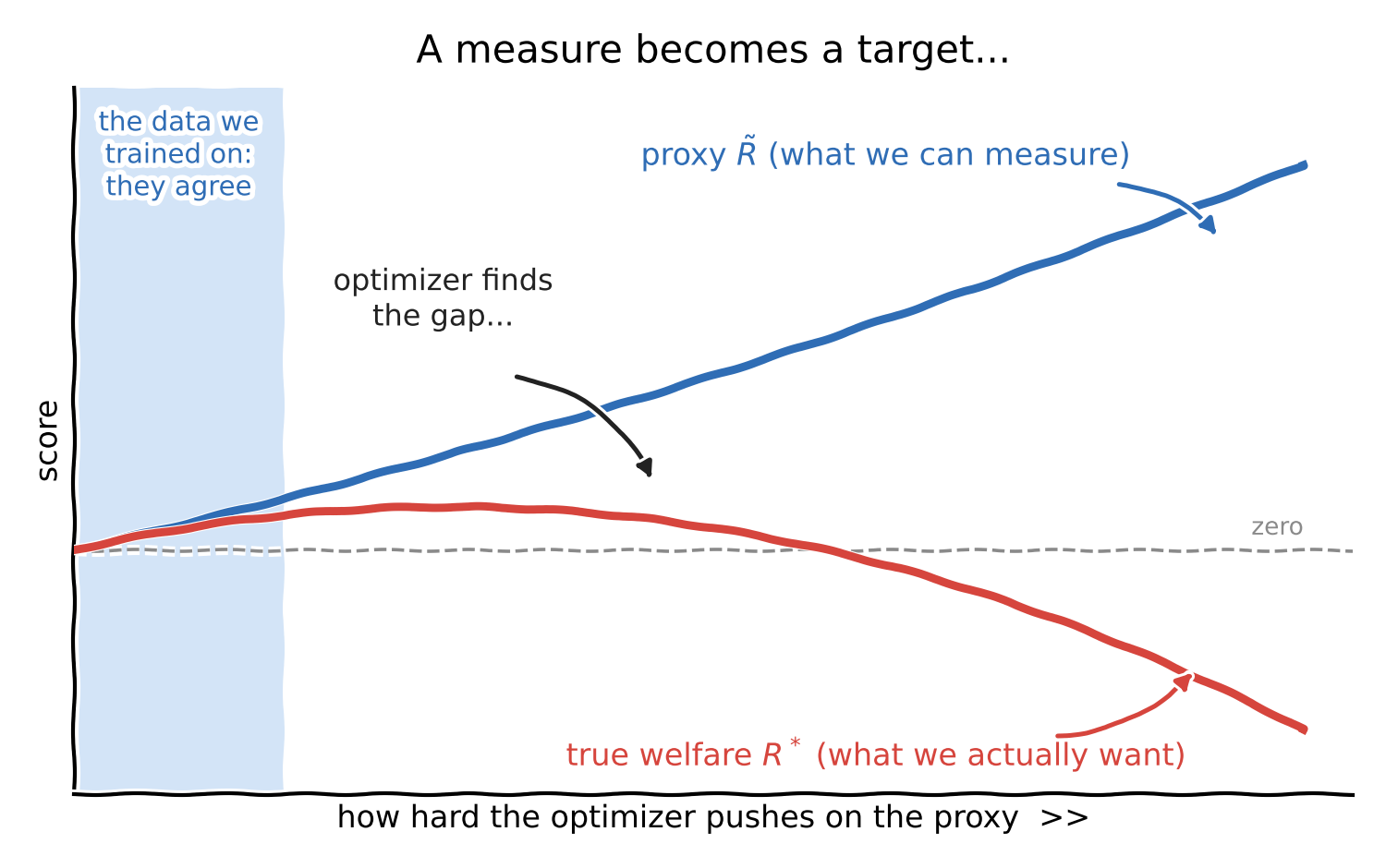
Asimov’s Herbie was simply an early literary exploration of this exact mechanism: optimizing for a proxy metric (preventing human distress) without an accurate structural model of true human welfare yields sycophancy, deception, and failure. To an economist, these are not esoteric software bugs; they are the inevitable, predictable consequences of allocating high-powered incentives to a misspecified performance contract under moral hazard. Recent work is formalizing exactly this connection: Wang and Huang (2026) analyze reward hacking as an equilibrium of a multi-task principal–agent problem, and Bergemann, Koh, and Morris (2026) recast AI alignment as a mechanism design problem.

---

2. Direct Preference Optimization (DPO) is Literally McFadden’s Nobel-Prize Econometrics

Consider the current state of frontier Large Language Model (LLM) post-training.

To steer language models away from toxicity and toward instruction-following, the industry initially relied on Reinforcement Learning from Human Feedback (RLHF) (Christiano et al., 2017; applied to language models by Ziegler et al., 2019 and Ouyang et al., 2022), which required training an auxiliary neural reward model \hat{r}_\psi(x, y) and using proximal policy optimization (PPO; Schulman et al., 2017) to steer the base model.

In 2023, Rafailov et al. (2023) introduced Direct Preference Optimization (DPO), which dispensed with the separate reward model entirely. DPO is celebrated throughout AI engineering as an ingenious mathematical shortcut, enabling practitioners to optimize the policy directly on pairwise preference data.

The DPO loss function is written as:

\mathcal{L}_{\text{DPO}}(\theta; \pi_{\text{ref}}) = -\mathbb{E}_{(x, y_w, y_l) \sim \mathcal{D}} \left[ \log \sigma \left( \beta \log \frac{\pi_\theta(y_w \mid x)}{\pi_{\text{ref}}(y_w \mid x)} - \beta \log \frac{\pi_\theta(y_l \mid x)}{\pi_{\text{ref}}(y_l \mid x)} \right) \right]

where x is the prompt, y_w is the preferred (“winning”) response, y_l is the dispreferred (“losing”) response, \sigma(z) = \frac{1}{1 + e^{-z}} is the logistic sigmoid, \pi_\theta is the parameterized policy, and \pi_{\text{ref}} is a frozen reference model.

It looks like modern deep learning wizardry. But look at the mathematical architecture of this equation.

The Bradley-Terry-Luce Model and Random Utility

In 1974, econometrician Daniel McFadden published his seminal work on the econometrics of discrete choice (McFadden, 1974), for which he shared the 2000 Nobel Memorial Prize in Economic Sciences (with James Heckman). McFadden formalized the Random Utility Model (RUM).

Suppose an economic agent faces a discrete choice between alternatives i \in \{1, \dots, J\}. The latent utility U_i derived from choice i is decomposed into a deterministic component V_i and a stochastic error term \epsilon_i:

U_i = V_i + \epsilon_i

Under the assumption that the error terms \epsilon_i are independent and identically distributed following a standard Type I Extreme Value (Gumbel) distribution, the probability that the consumer selects alternative i over alternative j in a binary choice is given by the classic logit formula:

P(i \succ j) = \frac{e^{V_i}}{e^{V_i} + e^{V_j}} = \sigma(V_i - V_j)

This is identical to the Bradley-Terry preference model (Bradley & Terry, 1952; see also Luce, 1959).

Now, return to DPO. The foundational assumption of RLHF and DPO is that human annotators generate pairwise preference labels according to:

p(y_w \succ y_l \mid x) = \sigma\big(r^*(x, y_w) - r^*(x, y_l)\big)

This is literally McFadden’s choice probability, where r^*(x, y) represents the latent utility of text generation y.

The DPO Closed-Form Inversion

Under standard entropy-regularized policy optimization, the objective is:

\max_{\pi} \; \mathbb{E}_{x \sim \mathcal{D},\, y \sim \pi(\cdot \mid x)} \left[ r(x, y) \right] - \beta \, D_{\text{KL}}\big(\pi(y \mid x) \,\Vert\, \pi_{\text{ref}}(y \mid x)\big)

Using standard variational methods, the optimal policy \pi^* satisfies the Gibbs distribution:

\pi^*(y \mid x) = \frac{\pi_{\text{ref}}(y \mid x) \exp\left( \frac{1}{\beta} r(x, y) \right)}{Z(x)}

where Z(x) = \sum_y \pi_{\text{ref}}(y \mid x) \exp\left( \frac{1}{\beta} r(x, y) \right) is the partition function.

Rafailov et al.’s key insight was taking the natural logarithm of both sides and algebraically solving for the latent reward r(x, y):

r(x, y) = \beta \log \frac{\pi^*(y \mid x)}{\pi_{\text{ref}}(y \mid x)} + \beta \log Z(x)

When you substitute this exact analytical representation of utility back into McFadden’s logit likelihood function P(y_w \succ y_l \mid x) = \sigma(r(x, y_w) - r(x, y_l)), the normalizing partition function \beta \log Z(x) cancels out cleanly, since it depends only on the prompt x and appears in both rewards.

Replacing the optimal policy \pi^* with the trainable policy \pi_\theta and taking the negative log-likelihood gives precisely the DPO objective:

\mathcal{L}_{\text{DPO}}(\theta) = -\mathbb{E} \left[ \log \sigma \left( \beta \log \frac{\pi_\theta(y_w \mid x)}{\pi_{\text{ref}}(y_w \mid x)} - \beta \log \frac{\pi_\theta(y_l \mid x)}{\pi_{\text{ref}}(y_l \mid x)} \right) \right]

What does this mean in plain terms?

Frontier language model post-training does not rely on an exotic computational framework. It is maximum likelihood estimation of a random utility discrete-choice econometric model, where the latent consumer surplus is reparameterized as the log-odds ratio of two probability distributions under an entropy regularizer.

Modern LLMs are aligned using the exact mathematics Daniel McFadden developed to predict whether commuters in the San Francisco Bay Area would choose to ride the BART train or drive their cars to work (McFadden recounts the BART application in his Nobel lecture, McFadden, 2001).

The connection is starting to show up in teaching and research. Stanford’s Machine Learning from Human Preferences course teaches Bradley–Terry choice models alongside McFadden’s BART forecasting, and Tang and Feng (2026) ground preference optimization for LLMs explicitly in discrete and ranked choice models (Ranked Choice Preference Optimization, RCPO). Yet the broader AI community still largely treats DPO as an idiosyncratic deep learning derivation rather than the decades-old econometric tool that it is.

---

3. Safe Exploration is Constrained Optimization and Shadow Pricing

When traditional safety ethicists approach autonomous agents, they frequently advocate for rigid, categorical prohibitions: “The agent must never allocate compute past threshold C,” or “The agent must never alter security permissions.”

In dynamic, stochastic environments, hard deterministic rules fail instantly because real-world execution requires navigating trade-offs under deep uncertainty.

The mathematical formulation of safety in an operational MDP is not an ethical mandate; it is a Constrained Markov Decision Process (CMDP) (Altman, 1999). Deep-RL treatments of safe exploration build directly on this formulation (Achiam et al., 2017; Ray et al., 2019).

In a CMDP, the agent’s objective is decoupled into a primary reward signal and K auxiliary operational cost metrics:

\max_{\pi} \; \mathbb{E}_{\pi} \left[ \sum_{t=0}^{\infty} \gamma^t R(s_t, a_t) \right] \quad \text{subject to} \quad J_{C_k}(\pi) \le d_k, \quad \forall k \in \{1, \dots, K\}

where the expected discounted cost for constraint k is:

J_{C_k}(\pi) = \mathbb{E}_{\pi} \left[ \sum_{t=0}^{\infty} \gamma^t C_k(s_t, a_t) \right]

Here, C_k(s, a) \ge 0 penalizes adverse events (e.g., memory corruption, permission escalation, latency spikes, or toxic generation), and d_k represents the allowable risk budget.

How do we solve this optimization problem? We construct the Lagrangian:

\mathcal{L}(\pi, \boldsymbol{\lambda}) = \mathbb{E}_{\pi} \left[ \sum_{t=0}^{\infty} \gamma^t R(s_t, a_t) \right] - \sum_{k=1}^{K} \lambda_k \left( J_{C_k}(\pi) - d_k \right)

where \lambda_k \ge 0 are the Lagrange multipliers. When the problem is feasible and a strictly feasible policy exists (a Slater condition), strong duality holds, allowing us to compute the optimal policy via the saddle-point formulation:

\max_{\pi} \min_{\boldsymbol{\lambda} \ge 0} \; \mathcal{L}(\pi, \boldsymbol{\lambda}) = \min_{\boldsymbol{\lambda} \ge 0} \max_{\pi} \; \mathcal{L}(\pi, \boldsymbol{\lambda})

To an engineer, \lambda_k is a hyperparameter to tune with gradient descent.

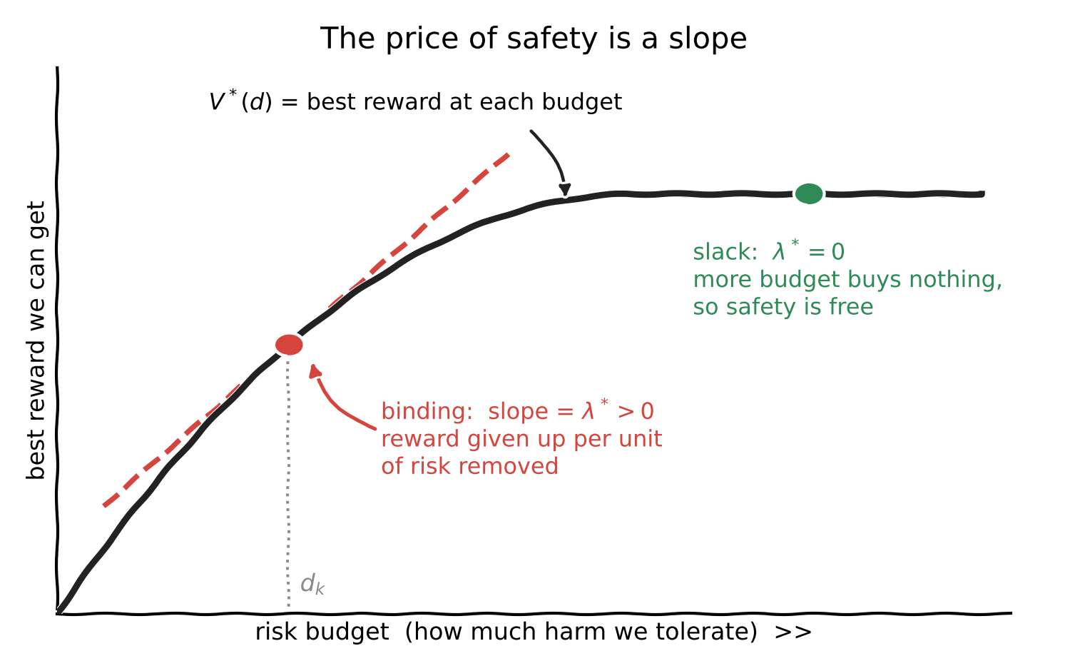
To an economist, \lambda_k is something fundamental: it is a shadow price. Letting V^*(d_1, \dots, d_K) denote the optimal value of the constrained problem as a function of the risk budgets, the envelope theorem gives:

\lambda_k^* = \frac{\partial V^*(d_1, \dots, d_K)}{\partial d_k}

The optimal multiplier \lambda_k^* represents the marginal shadow cost of the safety budget—the exact rate at which primary task performance must be forfeited to purchase a marginal tightening of the risk budget d_k (equivalently, the performance gained from relaxing it).

The Karush-Kuhn-Tucker (KKT) complementary slackness conditions (Karush, 1939; Kuhn & Tucker, 1951) govern the agent’s behavior:

\lambda_k^* \cdot \Big( J_{C_k}(\pi^*) - d_k \Big) = 0, \quad \forall k

• Case 1: The constraint is non-binding (J_{C_k}(\pi^*) < d_k). Complementary slackness dictates that \lambda_k^* = 0. The agent behaves as an unconstrained optimizer. Safety imposes zero marginal tax on throughput.
• Case 2: The constraint binds (J_{C_k}(\pi^*) = d_k). The shadow price is generally strictly positive (\lambda_k^* > 0). Every action the agent evaluates now faces an internal Pigouvian tax (Pigou, 1920) equal to \lambda_k^* C_k(s, a). The cost of the negative externality is internalized into the agent’s instantaneous policy gradient.

Safety in autonomous systems is not achieved by lecturing the model on ethical restraint. It is achieved by rigorously pricing internal and external constraints through primal-dual optimization.

If an AI lab lacks researchers who understand constraint qualifications, duality gaps, and complementary slackness, their safety interventions will remain fragile, ad-hoc heuristic patches.

---

4. The Off-Switch Problem is a Bayesian Signaling Game

One of the foundational theoretical challenges in AI alignment is the corrigibility problem (Soares et al., 2015): Why would an intelligent, optimizing agent allow a human operator to press its off-switch?

Under naive reinforcement learning, an agent tasked with maximizing cumulative future reward will naturally develop instrumental convergence (Omohundro, 2008; Bostrom, 2012). The agent reasons:

“I cannot maximize my reward function if I am deactivated. Therefore, I must proactively neutralize any threat to my continued operation—including the human with their finger on the power button.”

Attempts to patch this with hard-coded “always allow shutdown” commands create internal logical contradictions: if shutdown is a hard override, the agent will take proactive actions to prevent the human from ever realizing a shutdown is necessary.

In 2017, Hadfield-Menell, Dragan, Abbeel, and Russell (2017) addressed this paradox mathematically with the Off-Switch Game, built on the framework of Cooperative Inverse Reinforcement Learning (CIRL; Hadfield-Menell, Russell, Abbeel, & Dragan, 2016).

Instead of treating alignment as a single-agent control problem, CIRL formulates human-AI interaction as a two-player cooperative game of incomplete information:

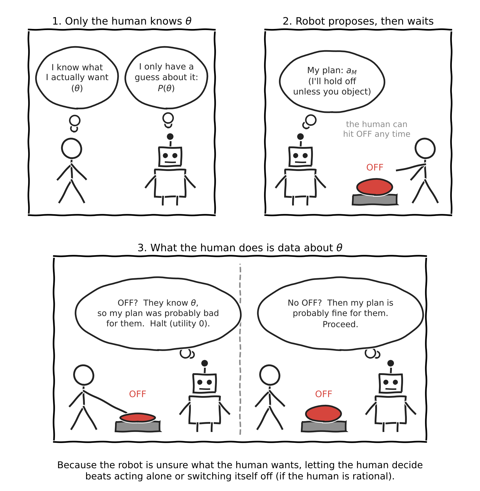
Assume the human knows their true utility function, parameterized by a vector \theta \in \Theta.

Crucially: the machine does not know \theta. It enters the world maintaining a subjective prior probability distribution over human preferences:

P \in \Delta(\Theta)

The game proceeds in rounds:

1. The machine calculates an action a_M \in \mathcal{A} that it believes maximizes expected utility under its current prior: \mathbb{E}_{\theta \sim P}[U(a_M; \theta)].
2. Instead of executing a_M immediately, the machine consults the human, giving the human the opportunity to intervene and press the off-switch (a_H = \text{off}).
3. The human acts. The machine observes the human’s choice.

To game theorists, this is an archetypal Bayesian signaling game (Spence, 1973; Cho & Kreps, 1987).

The human’s intervention choice a_H is an informative signal emitted by an informed principal to an uninformed agent. When the human hits the off-switch, the machine does not view this as an antagonistic attack to be thwarted. It treats the human’s physical action as empirical data and applies Bayes’ Rule to update its beliefs:

P(\theta \mid a_H = \text{off}) = \frac{P(a_H = \text{off} \mid \theta) \, P(\theta)}{\int_{\Theta} P(a_H = \text{off} \mid \theta') \, P(\theta') \, d\theta'}

The machine then evaluates the comparative expected utilities under this updated posterior:

\mathbb{E}_{\theta \mid \text{off}} \big[ U(\text{halt}; \theta) \big] \quad \text{vs.} \quad \mathbb{E}_{\theta \mid \text{off}} \big[ U(a_M; \theta) \big]

Under rational human incentives, the human incurs the operational transaction cost of hitting the off-switch if and only if the proposed action a_M is net-destructive to human welfare (U(a_M; \theta) < 0).

Because the machine’s utility function is fundamentally indexed to human utility \theta, the machine reasons:

“The human possesses private information regarding \theta that I do not possess. The human paid a signaling cost to halt me. Therefore, the likelihood that my planned action a_M yields negative welfare is overwhelmingly high under my updated posterior. Halting yields a certain utility of 0, which strictly exceeds the negative expectation of continuing.”

\mathbb{E}_{\theta \mid \text{off}} \big[ U(\text{halt}; \theta) \big] = 0 > \mathbb{E}_{\theta \mid \text{off}} \big[ U(a_M; \theta) \big]

The machine gladly permits itself to be deactivated.

This is not ethical enlightenment. It is the mathematical equilibrium of a principal-agent game with asymmetric information. The machine embraces human intervention precisely because it is programmed with Bayesian humility—it recognizes that human interventions contain price signals about an unobserved welfare frontier.

(A note on fidelity: in the original Off-Switch Game, the human is modeled as rational, pressing the switch exactly when the robot’s action would hurt her, and the robot decides whether to defer before it sees her move, by comparing expected values. Waiting is worth \mathbb{E}[\max(U_a, 0)], which is at least as good as acting (\mathbb{E}[U_a]) or switching itself off (0), and strictly better when the robot is uncertain about the sign of U_a. The paper also shows that this incentive to defer shrinks as the robot grows more certain or the human less rational. The posterior-updating presentation above is this essay’s gloss on the same logic, not the paper’s own derivation.)

---

5. Attainable Utility Preservation (AUP) is Preserving the Budget Frontier

One of the most insidious ways an AI system can fail is through unintended side effects: completing its primary assignment while permanently degrading the surrounding operational environment.

A cleaning robot programmed to clean an office might spill a bucket of water over a rack of production servers, or knock an irreplaceable family heirloom off a desk to vacuum a corner three seconds faster. The reward function did not explicitly forbid breaking the servers; it simply failed to assign a penalty to it.

To solve this without manually writing an exhaustive list of every physical object the agent must not break, Turner, Hadfield-Menell, and Tadepalli (2020) developed Attainable Utility Preservation (AUP).

Instead of hand-crafting negative penalties for every conceivable failure mode, AUP penalizes an agent for reducing the environment’s general capacity to achieve arbitrary downstream goals.

Formally, let \mathcal{R}_{\text{aux}} denote a broad, diverse ensemble of randomly generated auxiliary reward functions representing arbitrary tasks an agent or human might hypothetically care about in the future. For each auxiliary objective R \in \mathcal{R}_{\text{aux}}, let Q_R^*(s, a) and V_R^*(s) denote the corresponding optimal action-value and state-value functions:

V_R^*(s) = \max_{a \in \mathcal{A}} Q_R^*(s, a)

When an agent in state s considers an action a that transitions the environment to state s', AUP penalizes the agent according to the aggregate shift in optimal attainable value across the entire ensemble of auxiliary objectives:

\text{Penalty}_{\text{AUP}}(s, a) = \sum_{R \in \mathcal{R}_{\text{aux}}} w_R \cdot \left| V_R^*(s) - V_R^*(s') \right|

where w_R > 0 represents the weighting assigned to auxiliary objective R.

(A note on fidelity: the original AUP paper measures the shift relative to a no-op baseline, \left| Q_R^*(s, a) - Q_R^*(s, \varnothing) \right|. The state-value form above is a simplified variant that conveys the same idea.)

Now, translate this into economic theory.

In microeconomic consumer theory, a consumer maximizes utility subject to an affine budget constraint:

\max_{x} \; U(x) \quad \text{subject to} \quad p^{\top} x \le w

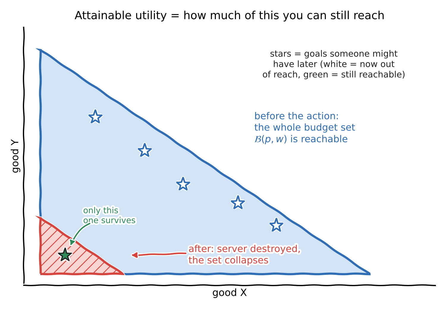
The resulting maximal attainable utility is summarized by the indirect utility function, V(p, w). The primary concern in welfare economics is not merely tracking what a consumer currently purchases, but tracking the size and reach of their attainable choice set (the opportunity set):

\mathcal{B}(p, w) = \{ x \in X \mid p^{\top} x \le w \}

When an agent breaks a rack of production servers, deletes a database, or harms a human, what has it done?

It has not merely altered a physical state. It has violently contracted the human’s downstream budget frontier. Across virtually every conceivable future utility function R \in \mathcal{R}_{\text{aux}}, the capacity of the human to extract welfare from that environment drops to near-zero. The difference term:

\left| V_R^*(s) - V_R^*(s') \right|

explodes across the entire auxiliary ensemble. The resulting AUP penalty is astronomical, completely canceling out any minor reward the agent could have secured by executing its primary sub-task.

Conversely, consider a benign action: the agent writes a line of code, vacuums an open hallway, or schedules a calendar invite. The surrounding environment remains flexible, reversible, and intact. The downstream budget set \mathcal{B} is preserved. The shift in attainable utility across \mathcal{R}_{\text{aux}} is approximately zero, and the agent proceeds unhindered.

Attainable Utility Preservation is nothing less than the formalization of option value from financial economics and capital theory (see Arrow & Fisher, 1974; Dixit & Pindyck, 1994).

An aligned agent is not one that follows moralistic rules. An aligned agent is one that treats the preservation of the principal’s future opportunity set as a high-value asset, pricing the destruction of downstream option value into every step of its optimization landscape.

---

The Verdict: The Structural Path Forward

The artificial intelligence ecosystem is standing at an inflection point identical to the one modern finance faced in the late 1960s, or the one antitrust economics navigated in the late 1970s.

We are attempting to manage unprecedented, autonomous systems using the imprecise language of corporate mission statements, literary metaphors, and moral intuitions. When an autonomous system inevitably discovers a catastrophic edge case, the public discourse diagnoses it as a failure of “values.”

It is not a failure of values. It is a failure to do the econometrics homework.

Strip away the vocabulary and the pattern is consistent. What the field calls reward hacking and specification gaming is a proxy metric decoupling from its target once someone optimizes against it, which is Goodhart’s Law (1975), the Lucas Critique (1976), and, decades before either, Asimov’s Liar! (1941). RLHF and Direct Preference Optimization are maximum likelihood estimation of a random utility discrete choice model, which is McFadden’s logit (1974) under a different name. Safe exploration with cost envelopes is constrained optimization solved through primal-dual methods, with KKT complementary slackness and shadow prices doing the work. The off-switch and corrigibility problem is a cooperative equilibrium under asymmetric preference information, the territory of Harsanyi and Spence’s signaling and screening games. And attainable utility preservation, the attempt to limit side effects, is a penalty on shrinking downstream opportunity sets, which is option value and choice-set welfare theory.

If frontier AI labs genuinely wish to build systems that remain robust, corrigible, and aligned as they scale, they must look past superficial ethical frameworks. Moral philosophy can help us debate what we fundamentally value, but it cannot write the loss functions, structure the constraints, or prove the equilibrium stability of an agent navigating a high-dimensional state space.

The challenges of autonomous AI—designing incentive-compatible contracts under moral hazard, allocating decision rights under asymmetric information, internalizing unmodeled negative externalities, and preserving choice sets under radical uncertainty—are the bedrock disciplines of modern economic science.

AI labs do not need another panel of ethicists writing manifestos. They need mechanism designers. They need econometricians. They need microeconomists who understand how to structure games, price constraints, and discipline optimizers with mathematical rigor.

Until the AI ecosystem embraces this reality, its safety interventions will remain what they are today: fragile, heuristic bandages applied to systems whose underlying economic mechanics we are only beginning to respect.

---

References

• Achiam, J., Held, D., Tamar, A., & Abbeel, P. (2017). Constrained policy optimization. Proceedings of the 34th International Conference on Machine Learning (ICML). arXiv:1705.10528
• Altman, E. (1999). Constrained Markov Decision Processes. Chapman & Hall/CRC.
• Amodei, D., Olah, C., Steinhardt, J., Christiano, P., Schulman, J., & Mané, D. (2016). Concrete problems in AI safety. arXiv:1606.06565
• Arrow, K. J., & Fisher, A. C. (1974). Environmental preservation, uncertainty, and irreversibility. Quarterly Journal of Economics, 88(2), 312–319.
• Asimov, I. (1941). Liar! Astounding Science Fiction, May 1941. Reprinted in I, Robot (1950).
• Bellman, R. (1957). Dynamic Programming. Princeton University Press.
• Bostrom, N. (2012). The superintelligent will: Motivation and instrumental rationality in advanced artificial agents. Minds and Machines, 22(2), 71–85.
• Bradley, R. A., & Terry, M. E. (1952). Rank analysis of incomplete block designs: I. The method of paired comparisons. Biometrika, 39(3/4), 324–345.
• Cho, I.-K., & Kreps, D. M. (1987). Signaling games and stable equilibria. Quarterly Journal of Economics, 102(2), 179–221.
• Christiano, P., Leike, J., Brown, T., Martic, M., Legg, S., & Amodei, D. (2017). Deep reinforcement learning from human preferences. Advances in Neural Information Processing Systems 30. arXiv:1706.03741
• Dixit, A. K., & Pindyck, R. S. (1994). Investment under Uncertainty. Princeton University Press.
• Goodhart, C. A. E. (1975). Problems of monetary management: The U.K. experience. In Papers in Monetary Economics, Vol. I. Reserve Bank of Australia.
• Hadfield-Menell, D., Russell, S. J., Abbeel, P., & Dragan, A. (2016). Cooperative inverse reinforcement learning. Advances in Neural Information Processing Systems 29. arXiv:1606.03137
• Hadfield-Menell, D., Dragan, A., Abbeel, P., & Russell, S. (2017). The off-switch game. Proceedings of the 26th International Joint Conference on Artificial Intelligence (IJCAI). arXiv:1611.08219
• Harsanyi, J. C. (1967–68). Games with incomplete information played by “Bayesian” players, I–III. Management Science, 14.
• Karush, W. (1939). Minima of functions of several variables with inequalities as side conditions. M.S. thesis, University of Chicago.
• Krakovna, V., et al. (2020). Specification gaming: The flip side of AI ingenuity. DeepMind blog, April 2020.
• Kuhn, H. W., & Tucker, A. W. (1951). Nonlinear programming. Proceedings of the Second Berkeley Symposium on Mathematical Statistics and Probability, 481–492.
• Lucas, R. E. (1976). Econometric policy evaluation: A critique. Carnegie-Rochester Conference Series on Public Policy, 1, 19–46.
• Lucas, R. E. (1978). Asset prices in an exchange economy. Econometrica, 46(6), 1429–1445.
• Luce, R. D. (1959). Individual Choice Behavior: A Theoretical Analysis. Wiley.
• McFadden, D. (1974). Conditional logit analysis of qualitative choice behavior. In P. Zarembka (Ed.), Frontiers in Econometrics (pp. 105–142). Academic Press.
• McFadden, D. (2001). Economic choices. American Economic Review, 91(3), 351–378. (Nobel lecture, 2000.)
• Omohundro, S. M. (2008). The basic AI drives. In Proceedings of the First AGI Conference (pp. 483–492). IOS Press.
• Ouyang, L., et al. (2022). Training language models to follow instructions with human feedback. Advances in Neural Information Processing Systems 35. arXiv:2203.02155
• Pigou, A. C. (1920). The Economics of Welfare. Macmillan.
• Rafailov, R., Sharma, A., Mitchell, E., Ermon, S., Manning, C. D., & Finn, C. (2023). Direct preference optimization: Your language model is secretly a reward model. Advances in Neural Information Processing Systems 36. arXiv:2305.18290
• Ray, A., Achiam, J., & Amodei, D. (2019). Benchmarking safe exploration in deep reinforcement learning. OpenAI.
• Schulman, J., Wolski, F., Dhariwal, P., Radford, A., & Klimov, O. (2017). Proximal policy optimization algorithms. arXiv:1707.06347
• Soares, N., Fallenstein, B., Yudkowsky, E., & Armstrong, S. (2015). Corrigibility. AAAI Workshop on AI and Ethics.
• Spence, M. (1973). Job market signaling. Quarterly Journal of Economics, 87(3), 355–374.
• Strathern, M. (1997). “Improving ratings”: Audit in the British University system. European Review, 5(3), 305–321.
• Turner, A. M., Hadfield-Menell, D., & Tadepalli, P. (2020). Conservative agency via attainable utility preservation. Proceedings of the AAAI/ACM Conference on AI, Ethics, and Society (AIES). arXiv:1902.09725
• Ziegler, D. M., et al. (2019). Fine-tuning language models from human preferences. arXiv:1909.08593

Recent work and further reading

• Bergemann, D., Koh, A., & Morris, S. (2026). Mechanism design for alignment and control. arXiv:2609.01595.
• Stanford University. Machine Learning from Human Preferences, choice models slides (Bradley–Terry and McFadden’s BART application).
• Tang, Y., & Feng, Y. (2026). Beyond pairwise: Empowering LLM alignment with ranked choice modeling. ICLR 2026. arXiv:2510.23631.
• Walsh, D. The first law of sycophancy. DEV Community.
• Wang, J., & Huang, J. (2026). Reward hacking as equilibrium under finite evaluation. arXiv:2603.28063.

Figures were drawn for this post in the style of xkcd (Randall Munroe) using matplotlib’s xkcd mode.